Sorting


 h ≥ (n/e)n which is Ω(n lg n)




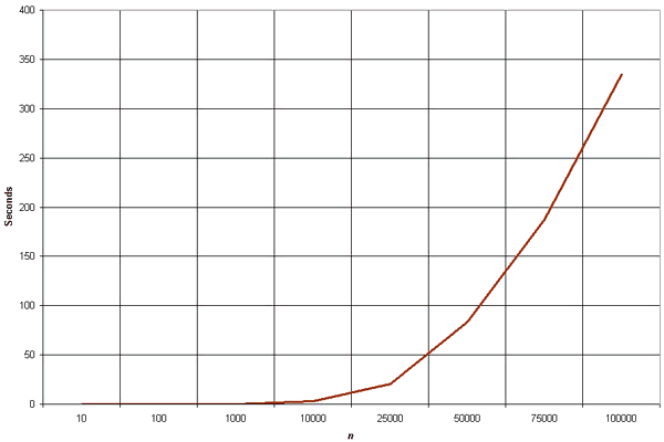


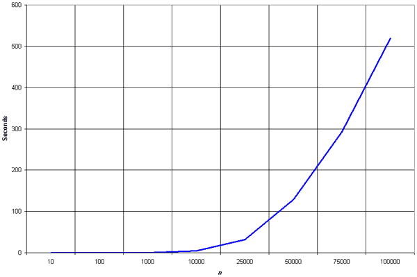

This algorithm is a simple extension of Insertion sort. Its speed comes from the fact that it exchanges elements that are far apart (the insertion sort exchanges only adjacent elements).
The idea of the Shell sort is to rearrange the file to give it the property that taking every hth element (starting anywhere) yields a sorted file. Such a file is said to be h-sorted.
The function form of the running time for all Shell sort depends on the increment sequence and is unknown. For the above algorithm, two conjectures are n(logn)2 andn1.25. Furthermore, the running time is not sensitive to the initial ordering of the given sequence, unlike Insertion sort.
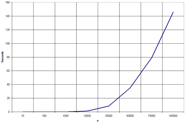
Shell sort is the method of choice for many sorting application because it has acceptable running time even for moderately large files and requires only small amount of code that is easy to get working. Having said that, it is worthwhile to replace Shell sort with a sophisticated sort in given sorting problem.


The binary heap data structures is an array that can be viewed as a complete binary tree. Each node of the binary tree corresponds to an element of the array. The array is completely filled on all levels except possibly lowest.
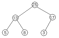
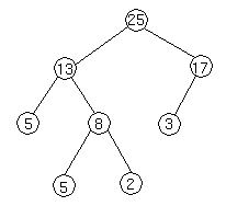
We represent heaps in level order, going from left to right. The array corresponding to the heap above is [25, 13, 17, 5, 8, 3].
The root of the tree A[1] and given index i of a node, the indices of its parent, left child and right child can be computed
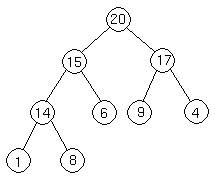
Let's try these out on a heap to make sure we believe they are correct. Take this heap,
 which is represented by the array [20, 14, 17, 8, 6, 9, 4, 1].
We'll go from the 20 to the 6 first. The index of the 20 is 1. To find the index of the left child, we calculate 1 * 2 = 2. This takes us (correctly) to the 14. Now, we go right, so we calculate 2 * 2 + 1 = 5. This takes us (again, correctly) to the 6.
Now let's try going from the 4 to the 20. 4's index is 7. We want to go to the parent, so we calculate 7 / 2 = 3, which takes us to the 17. Now, to get 17's parent, we calculate 3 / 2 = 1, which takes us to the 20.
A[PARENT (i)] ≥ A[i]
Thus, the largest element in a heap is stored at the root.
Following is an example of Heap:

By the definition of a heap, all the tree levels are completely filled except possibly for the lowest level, which is filled from the left up to a point. Clearly a heap of height hhas the minimum number of elements when it has just one node at the lowest level. The levels above the lowest level form a complete binary tree of height h -1 and 2h -1nodes. Hence the minimum number of nodes possible in a heap of height h is 2h. Clearly a heap of height h, has the maximum number of elements when its lowest level is completely filled. In this case the heap is a complete binary tree of height h and hence has 2h+1 -1 nodes.
Following is not a heap, because it only has the heap property - it is not a complete binary tree. Recall that to be complete, a binary tree has to fill up all of its levels with the possible exception of the last one, which must be filled in from the left side.
 lg n
lg n which is
  (lgn). This implies that an n-element heap has height
  lg n
lg n
In order to show this let the height of the n-element heap be h. From the bounds obtained on maximum and minimum number of elements in a heap, we get
 lgn
lgn .
.
We known from above that largest element resides in root, A[1]. The natural question to ask is where in a heap might the smallest element resides? Consider any path from root of the tree to a leaf. Because of the heap property, as we follow that path, the elements are either decreasing or staying the same. If it happens to be the case that all elements in the heap are distinct, then the above implies that the smallest is in a leaf of the tree. It could also be that an entire subtree of the heap is the smallest element or indeed that there is only one element in the heap, which in the smallest element, so the smallest element is everywhere. Note that anything below the smallest element must equal the smallest element, so in general, only entire subtrees of the heap can contain the smallest element.
Suppose we have a heap as follows
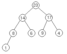
Let's suppose we want to add a node with key 15 to the heap. First, we add the node to the tree at the next spot available at the lowest level of the tree. This is to ensure that the tree remains complete.
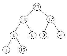
Let's suppose we want to add a node with key 15 to the heap. First, we add the node to the tree at the next spot available at the lowest level of the tree. This is to ensure that the tree remains complete.
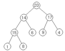
Now we do the same thing again, comparing the new node to its parent. Since 14 < 15, we have to do another swap:
Now we are done, because 15 20.
20.
Four basic procedures on heap are
It is important to note that swap may destroy the heap property of the subtree rooted at the largest child node. If this is the case, Heapify calls itself again using largest child node as the new root.
 (1) work), which is
  (lgn). Since we have a case in which Heapify's running time
  (lg n), its worst-case running time is Ω(lgn).
Example of Heapify
Suppose we have a complete binary tree somewhere whose subtrees are heaps. In the following complete binary tree, the subtrees of 6 are heaps:
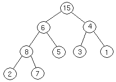

We then determine which of the three nodes is the greatest. If it is the root, we are done, because we have a heap. If not, we exchange the appropriate child with the root, and continue recursively down the tree. In this case, we exchange 6 and 8, and continue.
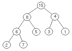
Now, 7 is greater than 6, so we exchange them.
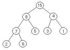
We are at the bottom of the tree, and can't continue, so we terminate.
 n/2
n/2 +1 . . n] are all leaves, the procedure BUILD_HEAP goes through the remaining nodes of the tree and runs 'Heapify' on each one. The bottom-up order of processing node guarantees that the subtree rooted at children are heap before 'Heapify' is run at their parent.
We can build a heap from an unordered array in linear time.
The HEAPSORT procedure takes time O(n lg n), since the call to BUILD_HEAP takes time O(n) and each of the n -1 calls to Heapify takes time O(lg n).
Now we show that there are at most én/2h+1ù nodes of height h in any n-element heap. We need two observations to show this. The first is that if we consider the set of nodes of height h, they have the property that the subtree rooted at these nodes are disjoint. In other words, we cannot have two nodes of height h with one being an ancestor of the other. The second property is that all subtrees are complete binary trees except for one subtree. Let Xh be the number of nodes of height h. Since Xh-1 o ft hese subtrees are full, they each contain exactly 2h+1 -1 nodes. One of the height h subtrees may not full, but contain at least 1 node at its lower level and has at least 2hnodes. The exact count is 1+2+4+ . . . + 2h+1 + 1 = 2h. The remaining nodes have height strictly more than h. To connect all subtrees rooted at node of height h., there must be exactly Xh -1 such nodes. The total of nodes is at least
In the conclusion, it is a property of binary trees that the number of nodes at any level is half of the total number of nodes up to that level. The number of leaves in a binary heap is equal to n/2, where n is the total number of nodes in the tree, is even and n/2
n/2 when n is odd. If these leaves are removed, the number of new leaves will be
  lg(n/2/2
 or
or  n/4
n/4 . If this process is continued for h levels the number of leaves at that level will be
  n/2h+1
 .
.





The basic version of quick sort algorithm was invented by C. A. R. Hoare in 1960 and formally introduced quick sort in 1962. It is used on the principle of divide-and-conquer. Quick sort is an algorithm of choice in many situations because it is not difficult to implement, it is a good "general purpose" sort and it consumes relatively fewer resources during execution.
Quick sort works by partitioning a given array A[p . . r] into two non-empty sub array A[p . . q] and A[q+1 . . r] such that every key in A[p . . q] is less than or equal to every key in A[q+1 . . r]. Then the two subarrays are sorted by recursive calls to Quick sort. The exact position of the partition depends on the given array and index q is computed as a part of the partitioning procedure.
Note that to sort entire array, the initial call Quick Sort (A, 1, length[A])
As a first step, Quick Sort chooses as pivot one of the items in the array to be sorted. Then array is then partitioned on either side of the pivot. Elements that are less than or equal to pivot will move toward the left and elements that are greater than or equal to pivot will move toward the right.
Partition selects the first key, A[p] as a pivot key about which the array will partitioned:
The running time of the partition procedure is (n) where n = r - p +1 which is the number of keys in the array.
Another argument that running time of PARTITION on a subarray of size (n) is as follows: Pointer i and pointer j start at each end and move towards each other, conveying somewhere in the middle. The total number of times that i can be incremented and j can be decremented is therefore O(n). Associated with each increment or decrement there are O(1) comparisons and swaps. Hence, the total time is O(n).
A very good partition splits an array up into two equal sized arrays. A bad partition, on other hand, splits an array up into two arrays of very different sizes. The worst partition puts only one element in one array and all other elements in the other array. If the partitioning is balanced, the Quick sort runs asymptotically as fast as merge sort. On the other hand, if partitioning is unbalanced, the Quick sort runs asymptotically as slow as insertion sort.
If the procedure 'Partition' produces two regions of size n/2. the recurrence relation is then
 (n2). The worst-case also occurs if A[1 . . n]starts out in reverse order.
In this version we choose a random key for the pivot. Assume that procedure Random (a, b) returns a random integer in the range [a, b); there are b-a+1 integers in the range and procedure is equally likely to return one of them. The new partition procedure, simply implemented the swap before actually partitioning.
Like other randomized algorithms, RANDOMIZED_QUICKSORT has the property that no particular input elicits its worst-case behavior; the behavior of algorithm only depends on the random-number generator. Even intentionally, we cannot produce a bad input for RANDOMIZED_QUICKSORT unless we can predict generator will produce next.
Worst-case
- Bubble Sort
- Insertion Sort
- Selection Sort
- Shell Sort
- Heap Sort
- Merge Sort
- Quick Sort
Sorting
The objective of the sorting algorithm is to rearrange the records so that their keys are ordered according to some well-defined ordering rule.
Problem: Given an array of n real number A[1.. n].
Objective: Sort the elements of A in ascending order of their values.
Internal Sort
If the file to be sorted will fit into memory or equivalently if it will fit into an array, then the sorting method is called internal. In this method, any record can be accessed easily.
External Sort
- Sorting files from tape or disk.
- In this method, an external sort algorithm must access records sequentially, or at least in the block.
Memory Requirement
- Sort in place and use no extra memory except perhaps for a small stack or table.
- Algorithm that use a linked-list representation and so use N extra words of memory for list pointers.
- Algorithms that need enough extra memory space to hold another copy of the array to be sorted.
Stability
A sorting algorithm is called stable if it is preserves the relative order of equal keys in the file. Most of the simple algorithm are stable, but most of the well-known sophisticated algorithms are not.
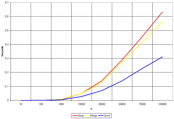
There are two classes of sorting algorithms namely, O(n2)-algorithms and O(n log n)-algorithms. O(n2)-class includes bubble sort, insertion sort, selection sort and shell sort. O(n log n)-class includes heap sort, merge sort and quick sort.
O(n2) Sorting Algorithms

O(n log n) Sorting Algorithms

Now we show that comparison-based sorting algorithm has an Ω(n log n) worst-case lower bound on its running time operation in sorting, then this is the best we can do. Note that in a comparison sort, we use only comparisons between elements to gain information about an input sequence <a1, a2, . . . , an>. That is, given two elementsai and aj we perform one of the tests, ai < aj, ai ≤ aj, ai = aj and ai ≥ aj to determine their relative order.
Given all of the input elements are distinct (this is not a restriction since we are deriving a lower bound), comparisons of the form ai = aj are useless, so no comparison ofai = aj are made. We also note that the comparison ai ≤ aj , ai ≥ aj and ai < aj are all equivalent. Therefore we assume that all comparisons have form ai ≥ aj.
The Decision Tree Model
Each time a sorting algorithm compares two elements ai and aj , there are two outcomes: "Yes" or "No". Based on the result of this comparison, the sorting algorithm may perform some calculation which we are not interested in and will eventually perform another comparison between two other elements of input sequence, which again will have two outcomes. Therefore, we can represent a comparison-based sorting algorithm with a decision tree T.
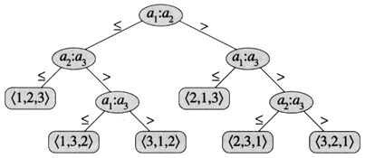
As an example, consider the decision tree for insertion sort operating on given elements a1, a2 and a3. There are are 3! = 6 possible permutations of the three input elements, so the decision tree must have at least 6 leaves.

In general, there are n! possible permutations of the n input elements, so decision tree must have at least n! leaves.
A Lower Bound for the Worst Case
The length of the longest path from the root to any of its leaves represents the worst-case number of comparisons the sorting algorithm perform. Consequently, the worst-case number of comparisons corresponds to the height of its tree. A lower bound on the height of the tree is therefore a lower bound on the running time of any comparison sort algorithm.
Theorem The running time of any comparison-based algorithm for sorting an n-element sequence is Ω(n lg n) in the worst case.
Examples of comparison-based algorithms (in CLR) are insertion sort, selection sort, merge sort, quicksort, heapsort, and treesort.
Proof Consider a decision tree of height h that sorts n elements. Since there are n! permutation of n elements and the tree must have at least n! leaves. We have
n! ≤ 2h
Taking logarithms on both sides
(lg(n!) ≤ h
 h ≥ lg(n!)
Taking logarithms on both sides
(lg(n!) ≤ h
Since the lg function is monotonically increasing, from Stirling's approximation we have
n! > (n/e)n where e = 2.71828 . . .
Bubble Sort
Bubble Sort is an elementary sorting algorithm. It works by repeatedly exchanging adjacent elements, if necessary. When no exchanges are required, the file is sorted.
SEQUENTIAL BUBBLESORT (A)
for i ← 1 to length [A] do
for j ← length [A] downto i +1 do
If A[A] < A[j-1] then
Exchange A[j] ↔ A[j-1]
Here the number of comparison made
1 + 2 + 3 + . . . + (n - 1) = n(n - 1)/2 = O(n2)
1 + 2 + 3 + . . . + (n - 1) = n(n - 1)/2 = O(n2)

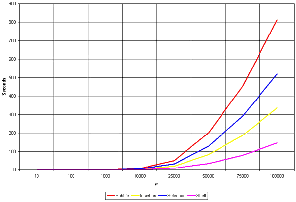
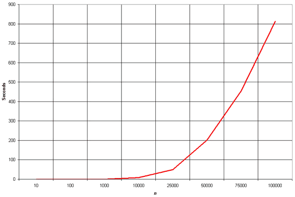
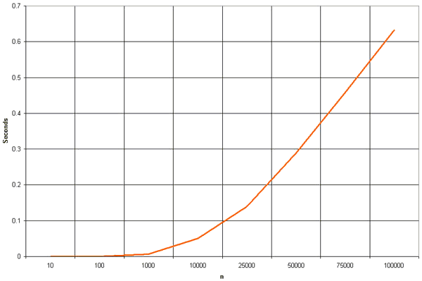
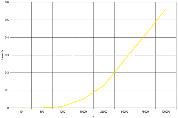
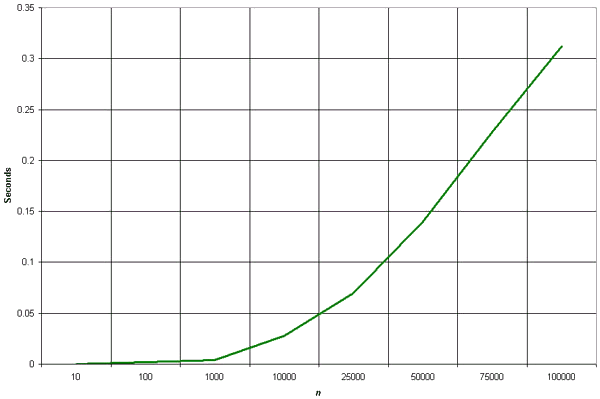
Clearly, the graph shows the n2 nature of the bubble sort.
In this algorithm the number of comparison is irrespective of data set i.e., input whether best or worst.
Memory Requirement
Clearly, bubble sort does not require extra memory.
Implementation
void bubbleSort(int numbers[], int array_size)
{
  int i, j, temp;

  for (i = (array_size - 1); i >= 0; i--)
  {
    for (j = 1; j <= i; j++)
    {
      if (numbers[j-1] > numbers[j])
      {
        temp = numbers[j-1];
        numbers[j-1] = numbers[j];
        numbers[j] = temp;
      }
    }
  }
}
Algorithm for Parallel Bubble Sort
PARALLEL BUBBLE SORT (A)
- For k = 0 to n-2
- If k is even then
- for i = 0 to (n/2)-1 do in parallel
- If A[2i] > A[2i+1] then
- Exchange A[2i] ↔ A[2i+1]
- Else
- for i = 0 to (n/2)-2 do in parallel
- If A[2i+1] > A[2i+2] then
- Exchange A[2i+1] ↔ A[2i+2]
- Next k
Parallel Analysis
Steps 1-10 is a one big loop that is represented n -1 times. Therefore, the parallel time complexity is O(n). If the algorithm, odd-numbered steps need (n/2) - 2processors and even-numbered steps require (n/2) - 1 processors. Therefore, this needs O(n) processors.
Insertion Sort
If the first few objects are already sorted, an unsorted object can be inserted in the sorted set in proper place. This is called insertion sort. An algorithm consider the elements one at a time, inserting each in its suitable place among those already considered (keeping them sorted). Insertion sort is an example of an incremental algorithm; it builds the sorted sequence one number at a time. This is perhaps the simplest example of the incremental insertion technique, where we build up a complicated structure on n items by first building it on n − 1 items and then making the necessary changes to fix things in adding the last item. The given sequences are typically stored in arrays. We also refer the numbers as keys. Along with each key may be additional information, known as satellite data. [Note that "satellite data" does not necessarily come from satellite!]
Algorithm: Insertion Sort
It works the way you might sort a hand of playing cards:
- We start with an empty left hand [sorted array] and the cards face down on the table [unsorted array].
- Then remove one card [key] at a time from the table [unsorted array], and insert it into the correct position in the left hand [sorted array].
- To find the correct position for the card, we compare it with each of the cards already in the hand, from right to left.
Note that at all times, the cards held in the left hand are sorted, and these cards were originally the top cards of the pile on the table.
Pseudocode
We use a procedure INSERTION_SORT. It takes as parameters an array A[1.. n] and the length n of the array. The array A is sorted in place: the numbers are rearranged within the array, with at most a constant number outside the array at any time.
INSERTION_SORT (A)
1. FOR j ← 2 TO length[A]
2. DO key ← A[j]
3. {Put A[j] into the sorted sequence A[1 . . j − 1]}
4. i ← j − 1
5. WHILE i > 0 and A[i] > key
6. DO A[i +1] ← A[i]
7. i ← i − 1
8. A[i + 1] ← key
2. DO key ← A[j]
3. {Put A[j] into the sorted sequence A[1 . . j − 1]}
4. i ← j − 1
5. WHILE i > 0 and A[i] > key
6. DO A[i +1] ← A[i]
7. i ← i − 1
8. A[i + 1] ← key
Example: Following figure (from CLRS) shows the operation of INSERTION-SORT on the array A= (5, 2, 4, 6, 1, 3). Each part shows what happens for a particular iteration with the value of j indicated. j indexes the "current card" being inserted into the hand.

Read the figure row by row. Elements to the left of A[j] that are greater than A[j] move one position to the right, and A[j] moves into the evacuated position.
Analysis
Since the running time of an algorithm on a particular input is the number of steps executed, we must define "step" independent of machine. We say that a statement that takes ci steps to execute and executed n times contributes cin to the total running time of the algorithm. To compute the running time, T(n), we sum the products of the cost and times column [see CLRS page 26]. That is, the running time of the algorithm is the sum of running times for each statement executed. So, we have
T(n) = c1n + c2 (n − 1) + 0 (n − 1) + c4 (n − 1) + c5 ∑2 ≤ j ≤ n ( tj )+ c6 ∑2 ≤ j ≤ n (tj − 1) + c7 ∑2 ≤ j ≤ n (tj − 1) + c8 (n − 1)
In the above equation we supposed that tj be the number of times the while-loop (in line 5) is executed for that value of j. Note that the value of j runs from 2 to (n − 1). We have
T(n) = c1n + c2 (n − 1) + c4 (n − 1) + c5 ∑2 ≤ j ≤ n ( tj )+ c6 ∑2 ≤ j ≤ n (tj − 1) + c7 ∑2 ≤ j ≤ n (tj − 1) + c8 (n − 1) Equation (1)
Best-Case
The best case occurs if the array is already sorted. For each j = 2, 3, ..., n, we find that A[i] less than or equal to the key when i has its initial value of (j − 1). In other words, when i = j −1, always find the key A[i] upon the first time the WHILE loop is run.
Therefore, tj = 1 for j = 2, 3, ..., n and the best-case running time can be computed using equation (1) as follows:
T(n) = c1n + c2 (n − 1) + c4 (n − 1) + c5 ∑2 ≤ j ≤ n (1) + c6 ∑2 ≤ j ≤ n (1 − 1) + c7 ∑2 ≤ j ≤ n (1 − 1) + c8 (n − 1)
T(n) = c1n + c2 (n − 1) + c4 (n − 1) + c5 (n − 1) + c8 (n − 1)
T(n) = (c1 + c2 + c4 + c5 + c8 ) n + (c2 + c4 + c5 + c8)
This running time can be expressed as an + b for constants a and b that depend on the statement costs ci. Therefore, T(n) it is a linear function of n.
The punch line here is that the while-loop in line 5 executed only once for each j. This happens if given array A is already sorted.
T(n) = an + b = O(n)
It is a linear function of n.
Worst-Case
The worst-case occurs if the array is sorted in reverse order i.e., in decreasing order. In the reverse order, we always find that A[i] is greater than the key in the while-loop test. So, we must compare each element A[j] with each element in the entire sorted subarray A[1 .. j − 1] and so tj = j for j = 2, 3, ..., n. Equivalently, we can say that since the while-loop exits because i reaches to 0, there is one additional test after (j − 1) tests. Therefore, tj = j for j = 2, 3, ..., n and the worst-case running time can be computed using equation (1) as follows:
T(n) = c1n + c2 (n − 1) + c4 (n − 1) + c5 ∑2 ≤ j ≤ n ( j ) + c6 ∑2 ≤ j ≤ n(j − 1) + c7 ∑2 ≤ j ≤ n(j − 1) + c8 (n − 1)
And using the summations in CLRS on page 27, we have
T(n) = c1n + c2 (n − 1) + c4 (n − 1) + c5 ∑2 ≤ j ≤ n [n(n +1)/2 + 1] + c6 ∑2 ≤ j ≤ n [n(n − 1)/2] + c7 ∑2 ≤ j ≤ n [n(n − 1)/2] + c8 (n − 1)
T(n) = (c5/2 + c6/2 + c7/2) n2 + (c1 + c2 + c4 + c5/2 − c6/2 − c7/2 + c8) n − (c2 + c4 + c5 + c8)
This running time can be expressed as (an2 + bn + c) for constants a, b, and c that again depend on the statement costs ci. Therefore, T(n) is a quadratic function of n.
Here the punch line is that the worst-case occurs, when line 5 executed j times for each j. This can happens if array A starts out in reverse order
T(n) = an2 + bn + c = O(n2)
It is a quadratic function of n.

The graph shows the n2 complexity of the insertion sort.
Worst-case and average-case Analysis
We usually concentrate on finding the worst-case running time: the longest running time for any input size n. The reasons for this choice are as follows:
- The worst-case running time gives a guaranteed upper bound on the running time for any input. That is, upper bound gives us a guarantee that the algorithm will never take any longer.
- For some algorithms, the worst case occurs often. For example, when searching, the worst case often occurs when the item being searched for is not present, and searches for absent items may be frequent.
- Why not analyze the average case? Because it's often about as bad as the worst case.
Example: Suppose that we randomly choose n numbers as the input to insertion sort.
On average, the key in A[j] is less than half the elements in A[1 .. j − 1] and it is greater than the other half. It implies that on average, the while loop has to look halfway through the sorted subarray A[1 .. j − 1] to decide where to drop key. This means that tj = j/2.
Although the average-case running time is approximately half of the worst-case running time, it is still a quadratic function of n.
Stability
Since multiple keys with the same value are placed in the sorted array in the same order that they appear in the input array, Insertion sort is stable.
Extra Memory
This algorithm does not require extra memory.
- For Insertion sort we say the worst-case running time is θ(n2), and the best-case running time is θ(n).
- Insertion sort use no extra memory it sort in place.
- The time of Insertion sort is depends on the original order of a input. It takes a time in Ω(n2) in the worst-case, despite the fact that a time in order of n is sufficient to solve large instances in which the items are already sorted.
Implementation
void insertionSort(int numbers[], int array_size)
{
int i, j, index;
for (i = 1; i < array_size; i++)
{
index = numbers[i];
j = i;
while ((j > 0) && (numbers[j − 1] > index))
{
numbers[j] = numbers[j − 1];
j = j − 1;
}
numbers[j] = index;
}
}
Selection Sort
This type of sorting is called "Selection Sort" because it works by repeatedly element. It works as follows: first find the smallest in the array and exchange it with the element in the first position, then find the second smallest element and exchange it with the element in the second position, and continue in this way until the entire array is sorted.
SELECTION_SORT (A)
for i ← 1 to n-1 do
min j ← i;
min x ← A[i]
for j ← i + 1 to n do
If A[j] < min x then
min j ← j
min x ← A[j]
A[min j] ← A [i]
A[i] ← min x
Selection sort is among the simplest of sorting techniques and it work very well for small files. Furthermore, despite its evident "naïve approach "Selection sort has a quite important application because each item is actually moved at most once, Section sort is a method of choice for sorting files with very large objects (records) and small keys.

The worst case occurs if the array is already sorted in descending order. Nonetheless, the time require by selection sort algorithm is not very sensitive to the original order of the array to be sorted: the test "if A[j] < min x" is executed exactly the same number of times in every case. The variation in time is only due to the number of times the "then" part (i.e., min j ← j; min x ← A[j] of this test are executed.
The Selection sort spends most of its time trying to find the minimum element in the "unsorted" part of the array. It clearly shows the similarity between Selection sort and Bubble sort. Bubble sort "selects" the maximum remaining elements at each stage, but wastes some effort imparting some order to "unsorted" part of the array. Selection sort is quadratic in both the worst and the average case, and requires no extra memory.
For each i from 1 to n - 1, there is one exchange and n - i comparisons, so there is a total of n -1 exchanges and (n -1) + (n -2) + . . . + 2 + 1 = n(n -1)/2comparisons. These observations hold no matter what the input data is. In the worst case, this could be quadratic, but in the average case, this quantity is O(n log n). It implies that the running time of Selection sort is quite insensitive to the input.
Implementation
void selectionSort(int numbers[], int array_size)
{
  int i, j;
  int min, temp;

  for (i = 0; i < array_size-1; i++)
  {
    min = i;
    for (j = i+1; j < array_size; j++)
    {
      if (numbers[j] < numbers[min])
        min = j;
    }
    temp = numbers[i];
    numbers[i] = numbers[min];
    numbers[min] = temp;
  }
}
Shell Sort
This algorithm is a simple extension of Insertion sort. Its speed comes from the fact that it exchanges elements that are far apart (the insertion sort exchanges only adjacent elements).
The idea of the Shell sort is to rearrange the file to give it the property that taking every hth element (starting anywhere) yields a sorted file. Such a file is said to be h-sorted.
SHELL_SORT (A)
for h = 1 to h £ N/9 do
for (; h > 0; h != 3) do
for i = h +1 to i £ n do
v = A[i]
j = i
while (j > h AND A[j - h] > v
A[i] = A[j - h]
j = j - h
A[j] = v
i = i + 1
The function form of the running time for all Shell sort depends on the increment sequence and is unknown. For the above algorithm, two conjectures are n(logn)2 andn1.25. Furthermore, the running time is not sensitive to the initial ordering of the given sequence, unlike Insertion sort.

Shell sort is the method of choice for many sorting application because it has acceptable running time even for moderately large files and requires only small amount of code that is easy to get working. Having said that, it is worthwhile to replace Shell sort with a sophisticated sort in given sorting problem.
Implementation
void shellSort(int numbers[], int array_size)
{
  int i, j, increment, temp;

  increment = 3;
  while (increment > 0)
  {
    for (i=0; i < array_size; i++)
    {
      j = i;
      temp = numbers[i];
      while ((j >= increment) && (numbers[j-increment] > temp))
      {
        numbers[j] = numbers[j - increment];
        j = j - increment;
      }
      numbers[j] = temp;
    }
    if (increment/2 != 0)
      increment = increment/2;
    else if (increment == 1)
      increment = 0;
    else
      increment = 1;
  }
}
Heap Sort
The binary heap data structures is an array that can be viewed as a complete binary tree. Each node of the binary tree corresponds to an element of the array. The array is completely filled on all levels except possibly lowest.

We represent heaps in level order, going from left to right. The array corresponding to the heap above is [25, 13, 17, 5, 8, 3].
The root of the tree A[1] and given index i of a node, the indices of its parent, left child and right child can be computed
PARENT (i)
return floor(i/2)
LEFT (i)
return 2i
RIGHT (i)
return 2i + 1
Let's try these out on a heap to make sure we believe they are correct. Take this heap,

We'll go from the 20 to the 6 first. The index of the 20 is 1. To find the index of the left child, we calculate 1 * 2 = 2. This takes us (correctly) to the 14. Now, we go right, so we calculate 2 * 2 + 1 = 5. This takes us (again, correctly) to the 6.
Now let's try going from the 4 to the 20. 4's index is 7. We want to go to the parent, so we calculate 7 / 2 = 3, which takes us to the 17. Now, to get 17's parent, we calculate 3 / 2 = 1, which takes us to the 20.
Heap Property
In a heap, for every node i other than the root, the value of a node is greater than or equal (at most) to the value of its parent.A[PARENT (i)] ≥ A[i]
Thus, the largest element in a heap is stored at the root.
Following is an example of Heap:

By the definition of a heap, all the tree levels are completely filled except possibly for the lowest level, which is filled from the left up to a point. Clearly a heap of height hhas the minimum number of elements when it has just one node at the lowest level. The levels above the lowest level form a complete binary tree of height h -1 and 2h -1nodes. Hence the minimum number of nodes possible in a heap of height h is 2h. Clearly a heap of height h, has the maximum number of elements when its lowest level is completely filled. In this case the heap is a complete binary tree of height h and hence has 2h+1 -1 nodes.
Following is not a heap, because it only has the heap property - it is not a complete binary tree. Recall that to be complete, a binary tree has to fill up all of its levels with the possible exception of the last one, which must be filled in from the left side.

Height of a node
We define the height of a node in a tree to be a number of edges on the longest simple downward path from a node to a leaf.Height of a tree
The number of edges on a simple downward path from a root to a leaf. Note that the height of a tree with n node isIn order to show this let the height of the n-element heap be h. From the bounds obtained on maximum and minimum number of elements in a heap, we get
2h ≤ n ≤ 2h+1-1
Where n is the number of elements in a heap.2h ≤ n ≤ 2h+1
Taking logarithms to the base 2
h ≤ lgn ≤ h +1
It follows that h = We known from above that largest element resides in root, A[1]. The natural question to ask is where in a heap might the smallest element resides? Consider any path from root of the tree to a leaf. Because of the heap property, as we follow that path, the elements are either decreasing or staying the same. If it happens to be the case that all elements in the heap are distinct, then the above implies that the smallest is in a leaf of the tree. It could also be that an entire subtree of the heap is the smallest element or indeed that there is only one element in the heap, which in the smallest element, so the smallest element is everywhere. Note that anything below the smallest element must equal the smallest element, so in general, only entire subtrees of the heap can contain the smallest element.
Inserting Element in the Heap
Suppose we have a heap as follows

Let's suppose we want to add a node with key 15 to the heap. First, we add the node to the tree at the next spot available at the lowest level of the tree. This is to ensure that the tree remains complete.

Let's suppose we want to add a node with key 15 to the heap. First, we add the node to the tree at the next spot available at the lowest level of the tree. This is to ensure that the tree remains complete.

Now we do the same thing again, comparing the new node to its parent. Since 14 < 15, we have to do another swap:

Now we are done, because 15
Four basic procedures on heap are
- Heapify, which runs in O(lg n) time.
- Build-Heap, which runs in linear time.
- Heap Sort, which runs in O(n lg n) time.
- Extract-Max, which runs in O(lg n) time.
Maintaining the Heap Property
Heapify is a procedure for manipulating heap data structures. It is given an array A and index i into the array. The subtree rooted at the children of A[i] are heap but node A[i] itself may possibly violate the heap property i.e., A[i] < A[2i] or A[i] < A[2i +1]. The procedure 'Heapify' manipulates the tree rooted at A[i] so it becomes a heap. In other words, 'Heapify' is let the value at A[i] "float down" in a heap so that subtree rooted at index i becomes a heap.Outline of Procedure Heapify
Heapify picks the largest child key and compare it to the parent key. If parent key is larger than heapify quits, otherwise it swaps the parent key with the largest child key. So that the parent is now becomes larger than its children.It is important to note that swap may destroy the heap property of the subtree rooted at the largest child node. If this is the case, Heapify calls itself again using largest child node as the new root.
Heapify (A, i)
- l ← left [i]
- r ← right [i]
- if l ≤ heap-size [A] and A[l] > A[i]
- then largest ← l
- else largest ← i
- if r ≤ heap-size [A] and A[i] > A[largest]
- then largest ← r
- if largest ≠ i
- then exchange A[i] ↔ A[largest]
- Heapify (A, largest)
Analysis
If we put a value at root that is less than every value in the left and right subtree, then 'Heapify' will be called recursively until leaf is reached. To make recursive calls traverse the longest path to a leaf, choose value that make 'Heapify' always recurse on the left child. It follows the left branch when left child is greater than or equal to the right child, so putting 0 at the root and 1 at all other nodes, for example, will accomplished this task. With such values 'Heapify' will called h times, where h is the heap height so its running time will be θ(h) (since each call doesExample of Heapify
Suppose we have a complete binary tree somewhere whose subtrees are heaps. In the following complete binary tree, the subtrees of 6 are heaps:
The Heapify procedure alters the heap so that the tree rooted at 6's position is a heap. Here's how it works. First, we look at the root of our tree and its two children.

We then determine which of the three nodes is the greatest. If it is the root, we are done, because we have a heap. If not, we exchange the appropriate child with the root, and continue recursively down the tree. In this case, we exchange 6 and 8, and continue.

Now, 7 is greater than 6, so we exchange them.

We are at the bottom of the tree, and can't continue, so we terminate.
Building a Heap
We can use the procedure 'Heapify' in a bottom-up fashion to convert an array A[1 . . n] into a heap. Since the elements in the subarray A[BUILD_HEAP (A)
- heap-size (A) ← length [A]
- For i ← floor(length[A]/2) down to 1 do
- Heapify (A, i)
We can build a heap from an unordered array in linear time.
Heap Sort Algorithm
The heap sort combines the best of both merge sort and insertion sort. Like merge sort, the worst case time of heap sort is O(n log n) and like insertion sort, heap sort sorts in-place. The heap sort algorithm starts by using procedure BUILD-HEAP to build a heap on the input array A[1 . . n]. Since the maximum element of the array stored at the root A[1], it can be put into its correct final position by exchanging it with A[n] (the last element in A). If we now discard node n from the heap than the remaining elements can be made into heap. Note that the new element at the root may violate the heap property. All that is needed to restore the heap property.HEAPSORT (A)
- BUILD_HEAP (A)
- for i ← length (A) down to 2 do
exchange A[1] ↔ A[i]
heap-size [A] ← heap-size [A] - 1
Heapify (A, 1)
The HEAPSORT procedure takes time O(n lg n), since the call to BUILD_HEAP takes time O(n) and each of the n -1 calls to Heapify takes time O(lg n).

Now we show that there are at most én/2h+1ù nodes of height h in any n-element heap. We need two observations to show this. The first is that if we consider the set of nodes of height h, they have the property that the subtree rooted at these nodes are disjoint. In other words, we cannot have two nodes of height h with one being an ancestor of the other. The second property is that all subtrees are complete binary trees except for one subtree. Let Xh be the number of nodes of height h. Since Xh-1 o ft hese subtrees are full, they each contain exactly 2h+1 -1 nodes. One of the height h subtrees may not full, but contain at least 1 node at its lower level and has at least 2hnodes. The exact count is 1+2+4+ . . . + 2h+1 + 1 = 2h. The remaining nodes have height strictly more than h. To connect all subtrees rooted at node of height h., there must be exactly Xh -1 such nodes. The total of nodes is at least
(Xh-1)(2h+1 + 1) + 2h + Xh-1 which is at most n.
Simplifying gives
Xh ≤ n/2h+1 + 1/2.
In the conclusion, it is a property of binary trees that the number of nodes at any level is half of the total number of nodes up to that level. The number of leaves in a binary heap is equal to n/2, where n is the total number of nodes in the tree, is even and
Implementation
void heapSort(int numbers[], int array_size)
{
  int i, temp;

  for (i = (array_size / 2)-1; i >= 0; i--)
    siftDown(numbers, i, array_size);

  for (i = array_size-1; i >= 1; i--)
  {
    temp = numbers[0];
    numbers[0] = numbers[i];
    numbers[i] = temp;
    siftDown(numbers, 0, i-1);
  }
}


void siftDown(int numbers[], int root, int bottom)
{
  int done, maxChild, temp;

  done = 0;
  while ((root*2 <= bottom) && (!done))
  {
    if (root*2 == bottom)
      maxChild = root * 2;
    else if (numbers[root * 2] > numbers[root * 2 + 1])
      maxChild = root * 2;
    else
      maxChild = root * 2 + 1;

    if (numbers[root] < numbers[maxChild])
    {
      temp = numbers[root];
      numbers[root] = numbers[maxChild];
      numbers[maxChild] = temp;
      root = maxChild;
    }
    else
      done = 1;
  }
}
Merge Sort
Merge sort is based on the divide-and-conquer paradigm. Its worst-case running time has a lower order of growth than insertion sort. Since we are dealing with subproblems, we state each subproblem as sorting a subarray A[p .. r]. Initially, p = 1 and r = n, but these values change as we recurse through subproblems.
To sort A[p .. r]:
1. Divide Step
If a given array A has zero or one element, simply return; it is already sorted. Otherwise, split A[p .. r] into two subarrays A[p .. q] and A[q + 1 .. r], each containing about half of the elements of A[p .. r]. That is, q is the halfway point of A[p .. r].
2. Conquer Step
Conquer by recursively sorting the two subarrays A[p .. q] and A[q + 1 .. r].
3. Combine Step
Combine the elements back in A[p .. r] by merging the two sorted subarrays A[p .. q] and A[q + 1 .. r] into a sorted sequence. To accomplish this step, we will define a procedure MERGE (A, p, q, r).
Note that the recursion bottoms out when the subarray has just one element, so that it is trivially sorted.
Algorithm: Merge Sort
To sort the entire sequence A[1 .. n], make the initial call to the procedure MERGE-SORT (A, 1, n).
MERGE-SORT (A, p, r)
1. IF p < r // Check for base case
2. THEN q = FLOOR[(p + r)/2] // Divide step
3. MERGE (A, p, q) // Conquer step.
4. MERGE (A, q + 1, r) // Conquer step.
5. MERGE (A, p, q, r) // Conquer step.
2. THEN q = FLOOR[(p + r)/2] // Divide step
3. MERGE (A, p, q) // Conquer step.
4. MERGE (A, q + 1, r) // Conquer step.
5. MERGE (A, p, q, r) // Conquer step.
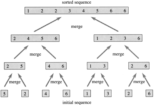
Example: Bottom-up view of the above procedure for n = 8.

Merging
What remains is the MERGE procedure. The following is the input and output of the MERGE procedure.
INPUT: Array A and indices p, q, r such that p ≤ q ≤ r and subarray A[p .. q] is sorted and subarray A[q + 1 .. r] is sorted. By restrictions on p, q, r, neither subarray is empty.
OUTPUT: The two subarrays are merged into a single sorted subarray in A[p .. r].
We implement it so that it takes Θ(n) time, where n = r − p + 1, which is the number of elements being merged.
Idea Behind Linear Time Merging
Think of two piles of cards, Each pile is sorted and placed face-up on a table with the smallest cards on top. We will merge these into a single sorted pile, face-down on the table.
A basic step:
- Choose the smaller of the two top cards.
- Remove it from its pile, thereby exposing a new top card.
- Place the chosen card face-down onto the output pile.
- Repeatedly perform basic steps until one input pile is empty.
- Once one input pile empties, just take the remaining input pile and place it face-down onto the output pile.
Each basic step should take constant time, since we check just the two top cards. There are at most n basic steps, since each basic step removes one card from the input piles, and we started with n cards in the input piles. Therefore, this procedure should take Θ(n) time.
Now the question is do we actually need to check whether a pile is empty before each basic step?
The answer is no, we do not. Put on the bottom of each input pile a special sentinel card. It contains a special value that we use to simplify the code. We use ∞, since that's guaranteed to lose to any other value. The only way that ∞ cannot lose is when both piles have ∞ exposed as their top cards. But when that happens, all the nonsentinel cards have already been placed into the output pile. We know in advance that there are exactly r − p + 1 nonsentinel cards so stop once we have performed r − p + 1 basic steps. Never a need to check for sentinels, since they will always lose. Rather than even counting basic steps, just fill up the output array from index p up through and including index r .
The answer is no, we do not. Put on the bottom of each input pile a special sentinel card. It contains a special value that we use to simplify the code. We use ∞, since that's guaranteed to lose to any other value. The only way that ∞ cannot lose is when both piles have ∞ exposed as their top cards. But when that happens, all the nonsentinel cards have already been placed into the output pile. We know in advance that there are exactly r − p + 1 nonsentinel cards so stop once we have performed r − p + 1 basic steps. Never a need to check for sentinels, since they will always lose. Rather than even counting basic steps, just fill up the output array from index p up through and including index r .
The pseudocode of the MERGE procedure is as follow:
MERGE (A, p, q, r )
1. n1 ← q − p + 1
2. n2 ← r − q
3. Create arrays L[1 . . n1 + 1] and R[1 . . n2 + 1]
4. FOR i ← 1 TO n1
5. DO L[i] ← A[p + i − 1]
6. FOR j ← 1 TO n2
7. DO R[j] ← A[q + j ]
8. L[n1 + 1] ← ∞
9. R[n2 + 1] ← ∞
10. i ← 1
11. j ← 1
12. FOR k ← p TO r
13. DO IF L[i ] ≤ R[ j]
14. THEN A[k] ← L[i]
15. i ← i + 1
16. ELSE A[k] ← R[j]
17. j ← j + 1
Example [from CLRS-Figure 2.3]: A call of MERGE(A, 9, 12, 16). Read the following figure row by row. Thats how we have done in the class.
- The first part shows the arrays at the start of the "for k ← p to r" loop, where A[p . . q] is copied into L[1 . . n1] and A[q + 1 . . r ] is
copied into R[1 . . n2]. - Succeeding parts show the situation at the start of successive iterations.
- Entries in A with slashes have had their values copied to either L or R and have not had a value copied back in yet. Entries in L and R with slashes have been copied back into A.
- The last part shows that the subarrays are merged back into A[p . . r], which is now sorted, and that only the sentinels (∞) are exposed in the arrays L and R.]

Running Time
The first two for loops (that is, the loop in line 4 and the loop in line 6) take Θ(n1 + n2) = Θ(n) time. The last for loop (that is, the loop in line 12) makes n iterations, each taking constant time, for Θ(n) time. Therefore, the total running time is Θ(n).
Analyzing Merge Sort
For simplicity, assume that n is a power of 2 so that each divide step yields two subproblems, both of size exactly n/2.
The base case occurs when n = 1.
When n ≥ 2, time for merge sort steps:
- Divide: Just compute q as the average of p and r, which takes constant time i.e. Θ(1).
- Conquer: Recursively solve 2 subproblems, each of size n/2, which is 2T(n/2).
- Combine: MERGE on an n-element subarray takes Θ(n) time.
Summed together they give a function that is linear in n, which is Θ(n). Therefore, the recurrence for merge sort running time is

Solving the Merge Sort Recurrence
By the master theorem in CLRS-Chapter 4 (page 73), we can show that this recurrence has the solution
T(n) = Θ(n lg n).
Reminder: lg n stands for log2 n.
Compared to insertion sort [Θ(n2) worst-case time], merge sort is faster. Trading a factor of n for a factor of lg n is a good deal. On small inputs, insertion sort may be faster. But for large enough inputs, merge sort will always be faster, because its running time grows more slowly than insertion sorts.
Recursion Tree
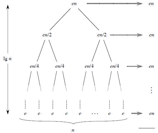
We can understand how to solve the merge-sort recurrence without the master theorem. There is a drawing of recursion tree on page 35 in CLRS, which shows successive expansions of the recurrence.
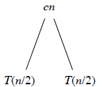
The following figure (Figure 2.5b in CLRS) shows that for the original problem, we have a cost of cn, plus the two subproblems, each costing T (n/2).

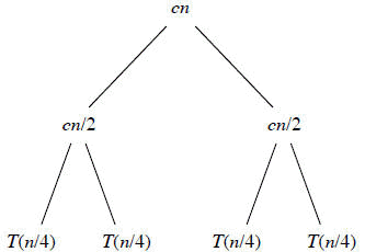
The following figure (Figure 2.5c in CLRS) shows that for each of the size-n/2 subproblems, we have a cost of cn/2, plus two subproblems, each costing T (n/4).

The following figure (Figure: 2.5d in CLRS) tells to continue expanding until the problem sizes get down to 1.

In the above recursion tree, each level has cost cn.
- The top level has cost cn.
- The next level down has 2 subproblems, each contributing cost cn/2.
- The next level has 4 subproblems, each contributing cost cn/4.
- Each time we go down one level, the number of subproblems doubles but the cost per subproblem halves. Therefore, cost per level stays the same.
The height of this recursion tree is lg n and there are lg n + 1 levels.
Mathematical Induction
We use induction on the size of a given subproblem n.
Base case: n = 1
Implies that there is 1 level, and lg 1 + 1 = 0 + 1 = 1.
Inductive Step
Our inductive hypothesis is that a tree for a problem size of 2i has lg 2i + 1 = i +1 levels. Because we assume that the problem size is a power of 2, the next problem size up after 2i is 2i + 1. A tree for a problem size of 2i + 1 has one more level than the size-2i tree implying i + 2 levels. Since lg 2i + 1 = i + 2, we are done with the inductive argument.
Total cost is sum of costs at each level of the tree. Since we have lg n +1 levels, each costing cn, the total cost is
cn lg n + cn.
Ignore low-order term of cn and constant coefÞcient c, and we have,
Θ(n lg n)
which is the desired result.

Implementation
void mergeSort(int numbers[], int temp[], int array_size){
m_sort(numbers, temp, 0, array_size - 1);
}
void m_sort(int numbers[], int temp[], int left, int right)
{
int mid;
if (right > left)
{
mid = (right + left) / 2;
m_sort(numbers, temp, left, mid);
m_sort(numbers, temp, mid+1, right);
merge(numbers, temp, left, mid+1, right);
}
}
void merge(int numbers[], int temp[], int left, int mid, int right)
{
int i, left_end, num_elements, tmp_pos;
left_end = mid - 1;
tmp_pos = left;
num_elements = right - left + 1;
while ((left <= left_end) && (mid <= right))
{
if (numbers[left] <= numbers[mid])
{
temp[tmp_pos] = numbers[left];
tmp_pos = tmp_pos + 1;
left = left +1;
}
else
{
temp[tmp_pos] = numbers[mid];
tmp_pos = tmp_pos + 1;
mid = mid + 1;
}
}
while (left <= left_end)
{
temp[tmp_pos] = numbers[left];
left = left + 1;
tmp_pos = tmp_pos + 1;
}
while (mid <= right)
{
temp[tmp_pos] = numbers[mid];
mid = mid + 1;
tmp_pos = tmp_pos + 1;
}
for (i = 0; i <= num_elements; i++)
{
numbers[right] = temp[right];
right = right - 1;
}
}
Quick Sort
The basic version of quick sort algorithm was invented by C. A. R. Hoare in 1960 and formally introduced quick sort in 1962. It is used on the principle of divide-and-conquer. Quick sort is an algorithm of choice in many situations because it is not difficult to implement, it is a good "general purpose" sort and it consumes relatively fewer resources during execution.
Good points
- It is in-place since it uses only a small auxiliary stack.
- It requires only n log(n) time to sort n items.
- It has an extremely short inner loop
- This algorithm has been subjected to a thorough mathematical analysis, a very precise statement can be made about performance issues.
Bad Points
- It is recursive. Especially if recursion is not available, the implementation is extremely complicated.
- It requires quadratic (i.e., n2) time in the worst-case.
- It is fragile i.e., a simple mistake in the implementation can go unnoticed and cause it to perform badly.
Quick sort works by partitioning a given array A[p . . r] into two non-empty sub array A[p . . q] and A[q+1 . . r] such that every key in A[p . . q] is less than or equal to every key in A[q+1 . . r]. Then the two subarrays are sorted by recursive calls to Quick sort. The exact position of the partition depends on the given array and index q is computed as a part of the partitioning procedure.
QuickSort
- If p < r then
- q Partition (A, p, r)
- Recursive call to Quick Sort (A, p, q)
- Recursive call to Quick Sort (A, q + r, r)
Note that to sort entire array, the initial call Quick Sort (A, 1, length[A])
As a first step, Quick Sort chooses as pivot one of the items in the array to be sorted. Then array is then partitioned on either side of the pivot. Elements that are less than or equal to pivot will move toward the left and elements that are greater than or equal to pivot will move toward the right.
Partitioning the Array
Partitioning procedure rearranges the subarrays in-place.PARTITION (A, p, r)
- x ← A[p]
- i ← p-1
- j ← r+1
- while TRUE do
- Repeat j ← j-1
- until A[j] ≤ x
- Repeat i ← i+1
- until A[i] ≥ x
- if i < j
- then exchange A[i] ↔ A[j]
- else return j
Partition selects the first key, A[p] as a pivot key about which the array will partitioned:
Keys ≤ A[p] will be moved towards the left .
Keys ≥ A[p] will be moved towards the right.
Keys ≥ A[p] will be moved towards the right.
The running time of the partition procedure is
Another argument that running time of PARTITION on a subarray of size
Array of Same Elements
Since all the elements are equal, the "less than or equal" teat in lines 6 and 8 in the PARTITION (A, p, r) will always be true. this simply means that repeat loop all stop at once. Intuitively, the first repeat loop moves j to the left; the second repeat loop moves i to the right. In this case, when all elements are equal, each repeat loop moves i andj towards the middle one space. They meet in the middle, so q= Floor(p+r/2). Therefore, when all elements in the array A[p . . r] have the same value equal toFloor(p+r/2).Performance of Quick Sort
The running time of quick sort depends on whether partition is balanced or unbalanced, which in turn depends on which elements of an array to be sorted are used for partitioning.A very good partition splits an array up into two equal sized arrays. A bad partition, on other hand, splits an array up into two arrays of very different sizes. The worst partition puts only one element in one array and all other elements in the other array. If the partitioning is balanced, the Quick sort runs asymptotically as fast as merge sort. On the other hand, if partitioning is unbalanced, the Quick sort runs asymptotically as slow as insertion sort.
Best Case
The best thing that could happen in Quick sort would be that each partitioning stage divides the array exactly in half. In other words, the best to be a median of the keys inA[p . . r] every time procedure 'Partition' is called. The procedure 'Partition' always split the array to be sorted into two equal sized arrays.If the procedure 'Partition' produces two regions of size n/2. the recurrence relation is then
And from case 2 of Master theoremT(n) = T(n/2) + T(n/2) +(n)
= 2T(n/2) +(n)
T(n) =  (n lg n)
Worst case Partitioning
The worst-case occurs if given array A[1 . . n] is already sorted. The PARTITION (A, p, r) call always return p so successive calls to partition will split arrays of lengthn, n-1, n-2, . . . , 2 and running time proportional to n + (n-1) + (n-2) + . . . + 2 = [(n+2)(n-1)]/2 =
Randomized Quick Sort
In the randomized version of Quick sort we impose a distribution on input. This does not improve the worst-case running time independent of the input ordering.In this version we choose a random key for the pivot. Assume that procedure Random (a, b) returns a random integer in the range [a, b); there are b-a+1 integers in the range and procedure is equally likely to return one of them. The new partition procedure, simply implemented the swap before actually partitioning.
Now randomized quick sort call the above procedure in place of PARTITIONRANDOMIZED_PARTITION (A, p, r)
i ← RANDOM (p, r)
Exchange A[p] ↔ A[i]
return PARTITION (A, p, r)
RANDOMIZED_QUICKSORT (A, p, r)
If p < r then
q ← RANDOMIZED_PARTITION (A, p, r)
RANDOMIZED_QUICKSORT (A, p, q)
RANDOMIZED_QUICKSORT (A, q+1, r)
Like other randomized algorithms, RANDOMIZED_QUICKSORT has the property that no particular input elicits its worst-case behavior; the behavior of algorithm only depends on the random-number generator. Even intentionally, we cannot produce a bad input for RANDOMIZED_QUICKSORT unless we can predict generator will produce next.
Analysis of Quick sort
Worst-case
Let T(n) be the worst-case time for QUICK SORT on input size n. We have a recurrence
T(n) = max1≤q≤n-1 (T(q) + T(n-q)) +where q runs from 1 to n-1, since the partition produces two regions, each having size at least 1.(n) --------- 1
Now we guess that T(n) ≤ cn2 for some constant c.
Substituting our guess in equation 1.We get
Since the second derivative of expression q2 + (n-q)2 with respect to q is positive. Therefore, expression achieves a maximum over the range 1≤ q ≤ n -1 at one of the endpoints. This gives the bound max (q2 + (n - q)2)) 1 + (n -1)2 = n2 + 2(n -1).
T(n) = max1≤q≤n-1 (cq2 ) + c(n - q2)) +(n)
= c max (q2 + (n - q)2) +(n)
Continuing with our bounding of T(n) we get


0 comments